Categories
MATLAB

Denoising a noisy signal using a median & running mean filters

To eliminate any large spikes in this matlab dataset example, we need to first loop over and come up with the median but not all the data points (only the data points that are particularly large). To decide which values are particularly large, we need to come up with some kind of threshold. Then any values that are above that threshold get replaced by the median of some number of numbers around them. We can generate a histogram of all the data values to pick the threshold levels. We can assume by looking at the histogram which ones are the real data values with high peaks and which ones are the outliers. In this example from the generated histogram 2 threshold levels were set as: 5 (threshold1), -5 (threshold2). We require here 2 threshold levels since there is high spike noise on both the positive and negative vertical axis of the original signal. Any data values above threshold1 and below threshold2 is going to be noise and that has to be removed generating the filtered signal (filtsig).

Then using a running mean filter algorithm in the time domain to set each data point in the previous filtered signal (filtsig) to be an average of the surrounding points from this signal generating the cleaned signal (cleanedsignal). This filter is not an appropriate filter for all kinds of noise. This is really specific for when noise is distributed positive and negative relative to the signal of interest.

Every time we apply a temporal filter to the data, regardless of the type of filter, could set the edges ‘edge effects’ of the time series to be the original signal or set zeros or just ignore them. We usually have to figure out what’s the best way to deal with ‘edge effects’ on a case by case basis given our specific application. In this example zeros were set at the edges of this filter.

Here is the generated MATLAB code in a .pdf file that illustrates the above :

https://usercontent.one/wp/www.kevnugent.com/wp-content/uploads/2020/12/denoising_code.pdf?media=1712708755

Categories
FPGA

DSP functionality advantages implemented within FPGAs

FPGAs have emerged as a great choice for systems requiring high-performance DSP functionality. They can implement parallelism computation (allow to easily parallelize the computational-intensive portions of the design) eg for critical filtering functions in DSP-Microprocessor-based application, freeing the DSP processor to perform algorithmically complex operations.

FPGAs have embedded memory, DSP blocks, embedded multipliers & embedded processors (soft/hard) that are well suited for implementing DSP functions such as FIR filters, FFTs, Encoders/Decoders, Arithmetic functions etc.

Embedded DSP blocks (or DSP slices) provide other functionality such as Multiply and Accumulate (MAC), Multiply & Add (MultAdd), Addition/Subtraction etc that are common arithmetic operations in DSP functions.

The 7 series FPGA DSP48E1 slice is functionally equivalent and fully compatible with the Virtex-5/6 & contain a 25bit Pre-adder, 25x18bit two’s complement Multiplier, 48-bit Accumulator/Logic Unit, Pattern Detector & Pipeline registers. Two DSP48E1 slices and dedicated interconnect form a DSP48E1 tile. The block RAM in 7 series can be split into two 18K block RAMs.

The DSP slice within the UltraScale architecture is defined using the DSP48E2 primitive (backwards compatible with the 7 series FPGA DSP48E1 slice). It contains a 27bit Pre-adder, improved 27x18bit Multiplier, 48-bit Accumulator/Logic Unit, Pattern Detector & Pipeline registers. The DSP48E2 blocks use signed arithmetic implementation. One 36K Block RAM (can split into 2x18K Block RAM), CLBs / dedicated Interconnect & 2 DSP48E2 slices form each DSP tile. To best match the resource capabilities and to get the most efficient mapping, code must be written using signed values in the HDL source. For migration purposes, designs created for the 25×18 multiplier in the 7 series FPGAs may need to be sign extended for the 27×18 multiplier in the UltraScale architecture.

Applications of the DSP slice include: Fixed and floating point FFT functions, Systolic FIR filters, MultiRate FIR filters, CIC filters & Wide real/complex multipliers/accumulators.

In a typical filter application, incoming data samples combine with filter coefficients through carefully synchronized mathematical operations which are dependent on the filter type and implementation strategy and then move on to the next processing stage. If the data source and destination are analog signals, then the samples must first pass through an ADC and the results fed through a DAC. An Analog LPF could be used before the ADC to filter out any unwanted high-frequency content signals above FNyquist (=fs/2) entering the ADC and avoid aliasing. Various design tools are available to help select the ideal length of the eg Digital LPF and the coefficient values. Also, decimation (or downsampling) at the output of the ADC, if required, can be carried out inside the FIR (Digital LPF) filter itself.

The goal is to select the appropriate parameters to achieve the required filter performance. The most popular design tool for choosing these parameters is MATLAB. [ FFi see my post :
https://www.kevnugent.com/2020/10/18/matlab-blogpost_005/ ]

The embedded memory in FPGAs meets external memory requirements and also eliminates the need for external memory devices in certain cases.

Embedded processors in FPGAs provide overall system integration & flexibility while partitioning the system between hardware & software. Designers can implement the system software components in the Embedded Processing System (PS) & implement hardware components in the FPGA Programmable Logic resources (PL).

FPGAs can implement Hardware Accelerators for each application allowing the designer to achieve best performance from Hardware Acceleration. The designer can implement hardware acceleration blocks by designing such blocks using parameterizable IP blocks or from scratch using HDL.

IP cores for Hardware acceleration could be : General cores (eg FIR, IIR), Modulation cores (eg QPSK, Equilizer etc), Encryption cores (eg DES), Error Correction cores ( eg Convolutional Encoder/Viterbi Decoder, CRC, Reed Solomon Encoder/Decoder etc)

This provides maximum flexibility, allowing designers to customize IP without changing a designs source code. Designers can integrate a parameterized IP core in HDL, can also port the IP to new FPGA families leading to a higher performance & lower cost.

If the system sample rate is below few KHz and is a single channel implementation, the DSP processor may be the obvious choice. However, as sample rates increase beyond a couple of MHz or if the system requires more than one single channel, FPGAs become more and more attractive. This means in a multiple-channel or high speed system we can take advantage of the parallelism within the FPGA device to maximize performance.

The DSP processor falls behind in raw data processing power for certain data intensive DSP functions such as Convolutional Encoding/Viterbi Decoding & FIR filters. At high data rates, the DSP may struggle to capture, process and output the data without any loss. This is due to the many shared resources, buses and even the core within the processor. The FPGA, however can dedicate resources to each of these functions.

DSPs are instruction based, not clock based. Typically 3-4 instructions are required for any mathematical operation on a single sample. The data must first be captured at the input, then forwarded to the processing core, cycled through that core for each operation and then released through the output.

There is also no level of customization for the design needs on DSP processor devices eg Hardware Accelerator (Co-processor) block such as Viterbi Co-processor, turbo co-processor & Enhanced Filter coprocessor. Such hardware blocks are fixed. DSP processors only allow a limited number of multipliers. Various DSP applications use external memory devices to manage large amounts of data processing. MAC operation is usually the performance bottleneck in most DSP applications.

In contrast, the FPGA is clock based, so every clock cycle has the potential ability to perform a mathematical operation on the incoming data stream.

Categories
Verilog coding styles

Verilog ‘if-else’ vs ‘case’ statements

Case’ statements in verilog or VHDL are more efficient than using ‘if-else‘ statements for parallel processing of data because ‘if-else’ can generate long combinatorial chains (priority scheme) of logic that can cause difficulties meeting timing.

It is worth noting here that the options of the ‘case’ statement must be mutually exclusive and all possible input values of the control expression must be included in the set of options (ie no incomplete assignments) to avoid the inference of unintended latches.

The following verilog code :

Will be synthesized to the following priority combinatorial logic :

All possible input values of the control expression must be included in the set of options (as shown above) to avoid the inference of unintended / accidental transparent latches.

However, if we recode the above verilog code to the following, it will direct the synthesis tool to implement parallel logic (fig2) rather than a priority scheme (fig1).

This will be synthesized to one multiplexer :

If a priority encoder is required (eg designing a priority interrupt control logic) this can be coded by using the nested if-else statements but need to be cautious & make sure that it will pass timing during synthesis at the maximum operating frequency of interest otherwise it will require re-designing/re-coding to try to resolve the timing issues.

Categories
Verilog coding styles

Verilog Blocking & Non-Blocking assignments elaborated

Blocking / Non-Blocking assignment rules

The main reason to use either Blocking or Non-Blocking assignments is to generate either combinational or sequential logic.

In non-blocking assignments (<=), all registers inside the always block are updated at the end. In blocking assignments (=), the registers are updated immediately.

Whether or not a flip-flop is inferred from a blocking assignment depends on whether or not the value of the variable being assigned needs to be remembered from one clock edge to the next.

It is good practice to separate combinational and sequential code as much as possible. In verilog, if we want to create sequential logic can use a clocked always block with non-blocking assignments. If on the other hand we want to create combinational logic can use an always block with blocking assignments. Best not to mix the two in the same always block but if they are mixed, need to be careful when doing this. Its up to the synthesis tools to determine whether a blocking assignment within a clocked always block will infer a flip-flop or not. If the signal is read before being assigned (eg fig2 below), the tools will infer sequential logic.

For simplicity purposes only showing in the verilog examples below the Always Block. These Always blocks are blocks of sequential logic since it involves a clock.

If on an active clock edge, the variable tmp is being assigned a value before it’s value is used (ie ‘write before read’ case) then no flip-flop is required & synthesis will not infer it as shown in fig1 below.

fig1

If the value of the reg is used before a new value is assigned to it (ie ‘read before write’ case), then the value that is used will be the value that was assigned on a previous clock. Therefore a flip-flop is required here as shown in fig2 below.

fig2

If all non-blocking assignments are used within the always block, it will look like :

or :

This image has an empty alt attribute; its file name is image-2.png
fig3

Non-blocking assignments always imply flip-flops (order of assignments doesn’t matter). Same block diagram is inferred on both cases as shown in fig3 above. They result in simultaneous or parallel statement execution.

Categories
DSP

Decimal number to Fixed-point & Floating-point Single/Double binary precision

213.3

213 -> ‘11010101’

0.3 -> ?

0.3 -> ‘01 0011 0011 0011 ….

Decimal number to fixed-point binary precision

From the above information 213.3 can be represented as follows :

In Fixed point the numbers are represented with a fixed number of digits after and sometimes before the decimal point eg fixed<11,3> denotes an 11-bit fixed point number of which 3 right most bits are fractional. eg real bit pattern number 11010101.010 from the example above.

How to represent this decimal number in IEEE 754 32-bit (single) floating-point notation?

In floating-point single (32-bits) or double (64-bits) precision, the number is represented with a mantissa and an exponent. The placement of the decimal point can float relative to the significant digits of the number.

Decimal number to floating-point single (32-bits) binary precision

For a 32-bit floating-point notation, need to express it in the form :

  • 1 sign bit, 8 exponent bits, 23 fraction bits

Shift the fixed-point binary representation 7 times to the left to represent the number as a scientific notation using mantissa (affects accuracy) & exponent (affects range) :

In 8-bit exponent the largest integer we can store is 2^8-1 = 255

Exponents we want also negative to represent very small numbers. Instead of using 2’s complement IEEE decided to bias the exponent.

Exponent bias (Expbias) = 2^(K-1) – 1

Since 8 exponent bits, K=8 . ExpBias = 2^7 – 1 = 127

The number here 213.3 is positive we add to the bias a value of 7 (E’=ExpBias+E=127 + 7=134dec) [134dec == ‘10000110’ binary]

Note: If sign bit = 0 (positive number) E’=E+ExpBias else E’=E-ExpBias

The number in IEEE754 32-bit floating point notation becomes :

How to represent this decimal number in IEEE 754 64-bit (double) floating-point notation?

Decimal number to floating-point single (64-bits) binary precision

For a 64-bit floating-point notation, need to express it in the form :

  • 1 sign bit, 11 exponent bits, 52 fraction bits

Since 11 exponent bits, K=11 . Exponent bias = 2^10 – 1 = 1023

Bias for double-precision format is 1023

The number 213.3 is positive we add to the bias a value of 7 (E’=ExpBias+E=1023+7=1030dec) [1030 dec == ‘10000000110’ binary]

The number in IEEE754 64-bit floating point notation becomes :

1153.125

1153 -> ‘10010000001’

.125 -> 0.001 (0*0.5 + 0*0.25 + 1*0.125)

Decimal number to fixed-point binary precision

From the above information 1153.125 can be represented as follows :

The above fixed point binary precision denotes a 14-bit fixed point number of which 3 right most bits are fractional

How to represent this decimal number in IEEE 754 32-bit (single) floating-point notation?

Decimal number to floating-point single (32-bits) binary precision

For a 32-bit floating-point notation, need to express it in the form :

  • 1 sign bit, 8 exponent bits, 23 fraction bits

Shift the fixed-point binary representation 10 times to the left to represent the number as a scientific notation using mantissa (affects accuracy) & exponent (affects range) :

Since 8 exponent bits, K=8 . Exponent bias = 2^7 – 1 = 127

The number here 1153.125 is positive we add to the bias a value of 10 (E’=ExpBias+E=127+10=137dec) [137dec == 10001001 binary]

The number in IEEE754 32-bit floating point notation becomes :

How to represent this decimal number in IEEE 754 64-bit (double) floating-point notation?

Decimal number to floating-point single (64-bits) binary precision

For a 64-bit floating-point notation, need to express it in the form :

  • 1 sign bit, 11 exponent bits, 52 fraction bits

Since 11 exponent bits, K=11 . Exponent bias = 2^10 – 1 = 1023

Bias for double-precision format is 1023

The number 1153.125 is positive we add to the bias a value of 10 (E’=ExpBias+E=1023+10=1033dec) [1033 dec == 10000001001 binary]

The number in IEEE754 64-bit floating point notation becomes :

Categories
MATLAB

FIR filter design using ‘Filter Builder’ App of System DSP / Fixed-Point Designer Toolboxes for Floating / Fixed-Point Arithmetic Precision..

DSP can be separated into 2 categories :

  • Fixed point precision
  • Floating point [ Single (32-bits) / Double (64-bits) ] precision

Fixed point DSPs are designed to represent and manipulate integers, positive and negative whole numbers typically via minimum of 16-bits yielding up to 2^16 possible bit patterns. In Fixed point the numbers are represented with a fixed number of digits after and sometimes before the decimal point.

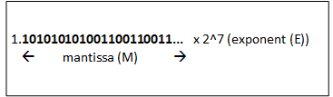
Floating point DSPs, on the other hand, represent and manipulate rational numbers via a minimum of 32-bits where the number is represented with a mantissa and an exponent yielding up to 2^32 bit patterns. In floating point, the placement of the decimal point can float relative to the significant digits of the number.

Floating point processors can support a much wider dynamic range of values than fixed point with the ability to represent very small numbers and very large numbers. They yield much greater precision than fixed-point processing and are ideally suited for computationally intensive applications or when computational accuracy is a critical requirement.

Each time a DSP generates a new number via a mathematical calculation that number must be rounded to the nearest value that can be then stored. Rounding &/or truncating numbers during signal processing naturally yields to quantization error or ‘noise’. Since the gaps between adjacent numbers can be much larger with fixed-point when compared to floating-point processing, round-off error can be much more pronounced.

It is generally easier to develop algorithms for floating-point DSPs as fixed-point algorithms require greater manipulation to compensate for quantization noise. Designers typically choose floating-point DSPs when implementing complex algorithms. Fixed point filters are commonly used in DSPs where data storage and power consumption are key limiting factors.

With the constraints we specify, Filter Builder App of the DSP System toolbox + Fixed-Point Designer toolbox software allows us to design efficient fixed-point filters.

Filter can be designed first for floating-point (single/double precision) input to obtain a baseline. Can then use the baseline for comparison with the fixed-point filter.

The filter for this example is a lowpass Equiripple FIR filter with the following specification :

  • Sample rate: 2kHz
  • Centre frequency: 650Hz
  • Transition Width: 100Hz
  • Equiripple Design
  • Maximum 1db of ripple in the passband
  • Minimum 80db of attenuation in the stopband

For a Centre frequency of 650Hz and Transition width of 100Hz :

  • Passband frequency : 600Hz
  • Stopband frequency : 700Hz

‘Filter Builder App’ is only installed when installing System DSP toolbox. When ‘System DSP toolbox’ is installed for MATLAB home edition, it automatically installs also ‘Signal Processing toolbox’ + ‘Filter Designer’ app.

To start designing the Filter using the ‘Filter Builder’ App, under APPS can click on the ‘Filter Builder’ and then select ‘Lowpass’.

It will be designed initially as a floating-point double precision data type :

Floating-point double precision (64-bits) data type

Within the 'Main' menu :

Save the variable as: LPF_Double_Precision

Filter specifications :

  • Impulse response: FIR
  • Order mode: Minimum
  • Filter type: Single-rate

Frequency specifications :

  • Frequency units: kHz
  • Input sample rate: 2
  • Passband frequency: 0.6
  • Stopband frequency: 0.7

Magnitude specifications :

  • Magnitude units: dB
  • Passband ripple: 1
  • Stopband attenuation: 80

Algorithm :

  • Design method: Equiripple
  • Design options (can leave default values here)

Filter implementation :

  • Structure: Direct-Form FIR

Within the Data types menu :

  • Arithmetic : Double precision

Need to select Apply button to apply the updated Main & Data Types settings before visualizing the design. Then select View Filter Response

This will display automatically the Magnitude Response (dB) because the Analysis option has already Magnitude Response (dB) option ticked by default. Under Analysis can also view manually other filter characteristics such as :

  • Phase Response
  • Magnitude and Phase Responses (together)
  • Impulse Response
  • Pole-Zero plot
  • Filter Coefficients
  • Filter Information
  • etc

Filter Information displays things such as :

  • Filter structure
  • Filter Length
  • Stable or not
  • Linear Phase or not
  • Design Algorithm
  • Design Options
  • Design Specifications
  • Measurements
  • Implementation Cost

From the Measurements info can see whether it met the design specification requirements. The Filter Structure displays the filter structure eg Direct-Form FIR, the Filter length, stability & linear phase status. The Implementation Cost displays the number of Multipliers/Adders/States used + Multiplications/Additions per Input Sample (ie it estimates the computational complexity).

In this example the Measurements, Filter Structure & Implementation Cost results of this Equiripple LPF FIR were :

Measurements :

  • Sample Rate: 2kHz => o.k
  • Passband Edge: 600Hz => o.k
  • 3-dB point: 616.3011Hz
  • 6-dB point: 628.1421Hz
  • Stopband Edge: 700Hz => o.k
  • Passband Ripple: 0.96726dB < 1dB => ok
  • Stopband Attenuation: 80.0905dB > 80dB => o.k
  • Transition Width: 100Hz => ok

Filter Structure & it’s properties :

  • Filter Structure : Direct-Form FIR
  • Filter Length : 51
  • Stable : Yes
  • Linear Phase : Yes (Type 1)

Implementation Cost :

  • Number of Multipliers: 51
  • Number of Adders: 50
  • Number of States: 50
  • Multiplications per Input Sample: 51
  • Additions per Input Sample: 50

Once satisfied with the Filter results,

Within the Code Generation menu :

Can generate MATLAB code (getFilter.m) based on filter specifications by selecting ‘Generate MATLAB code…’ option & leaving ‘Generate function that returns your filter as an output’ default option ticked.

Can also enquire automatically within the generated getFilter.m code the above results by adding manually the measure / info & cost functions. Then can also add the fvtool function to visualize the resulting design.

Here is the generated MATLAB code in a .pdf file that illustrates the above :

https://usercontent.one/wp/www.kevnugent.com/wp-content/uploads/2020/10/FIR_LPF_Floating_Double_Precision.pdf?media=1712708755

Floating-point single precision (32-bits) data type

Same steps were followed as above apart from the following :

Within the 'Main' menu :

Save the variable as: LPF_Single_Precision

Within the Data types menu :

  • Arithmetic : Single precision

In this example the Measurements, Filter Structure & Implementation Cost results were identical and not much difference in Magnitude response between Single-Precision and Double Precision.

Here is the generated MATLAB code in a .pdf file that illustrates the above :

https://usercontent.one/wp/www.kevnugent.com/wp-content/uploads/2020/10/FIR_LPF_Floating_Single_Precision.pdf?media=1712708755

Fixed-point full precision data type (initial default settings)

Note: ‘Fixed-point Designer’ toolbox is required here for the ‘Fixed point’ option to be visible under the Data types Arithmetic menu.

Within the 'Main' menu leave same settings as above apart from :

Save the variable as: LPF_Fixed_Point

Within the Data types menu :

Arithmetic : Fixed point

Fixed point data types : (leave all default values here)

Input Word Length: 16 (default value)
Input Frac Length: 15 (default value)

Coefficient Word Length: 16 (default value)
Filter intervals : Full Precision (default value)

Select the Apply button to apply the updated Main & Data Types settings before visualizing the design. Then select View Filter Response

In this example the Measurements/Implementation Cost results of this Equiripple LPF FIR were :

Measurements :

  • Sample Rate: 2kHz => o.k
  • Passband Edge: 600Hz => o.k
  • 3-dB point: 616.304Hz
  • 6-dB point: 628.144Hz
  • Stopband Edge: 700Hz => o.k
  • Passband Ripple: 0.9685dB < 1dB => ok
  • Stopband Attenuation: 72.576dB < 80dB => Not o.k
  • Transition Width: 100Hz => ok

Filter Structure & it’s properties :

  • Filter Structure : Direct-Form FIR
  • Filter Length : 51
  • Stable : Yes
  • Linear Phase : Yes (Type 1)
  • Arithmetic : fixed
  • Filter Internals : Full Precision
  • Round Mode : No rounding
  • Overflow Mode : No overflow
  • etc

Implementation Cost :

  • Number of Multipliers: 51
  • Number of Adders: 50
  • Number of States: 50
  • Multiplications per Input Sample: 51
  • Additions per Input Sample: 50

This fails the Stopband Attenuation requirement of 80dB

Here is the generated MATLAB code in a .pdf file that illustrates the above :

https://usercontent.one/wp/www.kevnugent.com/wp-content/uploads/2020/10/FIR_LPF_Fixed_Point_original.pdf?media=1712708755

Fixed-point full precision data type (increasing the transition width from 100dB ->200dB)

If we want a high minimum stopband attenuation without compromising on the number of coefficient bits, we must relax the other filter design constraint: the transition width

Increasing just the transition width from 100kHz -> 200kHz within the Main menu as follows :

  • Passband frequency: 0.55 (Frequency units: kHz)
  • Stopband frequency: 0.75

and the same coefficient length of 16, enabled us to get a higher Stopband Attenuation of 73.0869dB but this is still < 80dB ie it still misses out the spec requirements for stopband attenuation.

For FIR filters in general, each bit of coefficient word length provides approximately 4.5 – 5dB of stopband attenuation. However, it was almost impossible to achieve more than 4.5dB per bit coefficient word length in this example, even after relaxing the transition width (as illustrated here).

The filter length in this instance also decreased from 51 to 27 implying that fewer taps are required to implement this new FIR filter.

Here is the generated MATLAB code in a .pdf file that illustrates the above :

https://usercontent.one/wp/www.kevnugent.com/wp-content/uploads/2020/10/FIR_LPF_Fixed_Point_incr_transition_width.pdf?media=1712708755

Fixed-point full precision data type (increasing the coefficient length from 16bits -> 24bits)

If the coefficient word length is flexible, within the Main menu we leave the original default settings i.e

  • Passband frequency: 0.6 (Frequency units: kHz)
  • Stopband frequency: 0.7

and within the Data Types we can increment the Coefficients word length from 16bits -> 24bits.

Increasing the number of bits allowed for the coefficient word length makes the quantization error smaller and enables us to match the design requirement for 80dB of Stopband Attenuation. For a coefficient word length of 24bits a Stopband Attenuation of 80.0904dB was achieved as shown in the following attached modified regenerated MATLAB code within the .pdf file :

https://usercontent.one/wp/www.kevnugent.com/wp-content/uploads/2020/10/FIR_LPF_Fixed_Point_incr_coefficient_word_length.pdf?media=1712708755

Its worth mentioning that in many fixed point design applications, the coefficient word length is not flexible eg if we are restricted to work with 14bits, from the results shown below, the requested minimum Stopband Attenuation of 80dB cannot be reached! A filter with 14-bit coefficient quantization can achieve a minimum of only 62.7048dB after reviewing the Filter Information/Measurements: Stopband Attenuation results as shown below:

Measurements :

  • Sample Rate: 2kHz => o.k
  • Passband Edge: 600Hz => o.k
  • 3-dB point: 616.3202Hz
  • 6-dB point: 628.1535Hz
  • Stopband Edge: 700Hz => o.k
  • Passband Ripple: 0.97369dB < 1dB => ok
  • Stopband Attenuation: 62.7048dB < 80dB => Not o.k
  • Transition Width: 100Hz => ok

Here is the generated MATLAB code in a .pdf file that illustrates the above :

https://usercontent.one/wp/www.kevnugent.com/wp-content/uploads/2020/10/FIR_LPF_Fixed_Point_decr_coefficient_word_length.pdf?media=1712708755

Categories
MATLAB

Applying specification-based filter design methodology (using fdesign function) of the Signal Processing Toolbox

A recommended method for designing Filters in MATLAB using the Signal Processing Toolbox is to apply a specification-based filter design methodology using the fdesign function to create a filter design specification object that contains the specifications for a filter
such as :

  • Passband Ripple (amount of ripple or variation we allow in the passband)
  • Stopband Attenuation (reduction in signal we want in the stopband)
  • Passband Frequency (highest frequency we want to let through our filter)
  • Stopband Frequency (frequency beyond which we want to block all the frequencies in our filter)

We avoid a lot of trial & error by getting a list in MATLAB for all the design methods which are available to us, by using designmethods function to determine the filter design methods that work for the new filter specification object. Then, use the design function to design the filter from the filter design specifications object.

The class of digital filters may broadly be categorized into finite impulse response (FIR) and infinite impulse response (IIR) filters.

FIR filters are quite stable and their impulse response is of finite period (they settle to zero in finite time). As they do not use previous output values to compute their present output ie they have no feedback, they can never become unstable for any type of input signal which gives them distinct advantage over IIR filters. Most FIRs are linear phase filters. They are linear where the phase response of the filter is a linear (straight-line) function of frequency and this occurs if it’s coefficients are symmetrical around the center coefficient. They are generally chosen for applications where linear phase is important and a decent amount of memory and computational performance are available. If linear phase, no ‘phase distortion’ is introduced into the signal to be filtered as all frequencies are shifted in time by the same amount (ie constant phase delay). They also have fixed point performance advantages since the effects of quantization are less severe than that of an IIR. They are widely deployed in audio and biomedical signal enhancement applications.

IIR on the other hand will respond indefinitely (infinite nature of the impulse response). It can be viewed as 2 FIR filters, one of which is connected in a feedback loop. The feedback loop one is the ‘recursive’ section compared to the other ‘non-recursive’ one. Need to ensure that the ‘recursive’ section is stable. Therefore, an IIR filter has both poles and zeros and have to restrict all the poles (ie the ‘recursive’ part) inside the unit circle for the overall filter to be stable. The phase characteristics of an IIR filters are generally non-linear especially near the cut-off frequencies. They require more scaling and numeric overflow analysis when implemented in fixed point. It can have fewer components/less coefficients & memory (lower implementation cost) than FIR for frequency selective filter designs. They have been widely deployed in audio equalisation, biomedical sensor signal processing, IoT smart sensors and high-speed telecommunication/RF low latency applications due to their low number of coefficients.

An FIR ‘Equiripple’ Low Pass Filter (LPF) type in the MATLAB example below requires 175 multipliers & 174 adders compared to IIR ‘Ellip’ LPF which only requires 16 of each. So FIRs usually require many more coefficients for achieving a sharp cut-off than their IIR counterparts. The consequence of this is that they require much more memory and significantly a higher amount of MAC (Multiply-Accumulate) operations.

The longer the filter is, the more number of operations it takes to execute the filter when running it. The higher the order of the filter, the more arithmetic operations it takes and this leads to more hardware (number of adders, multipliers etc). We may want to compromise on the stopband attenuation for the sake of a lower filter order. However, the stopband attenuation is very important. We may have to trade it off for a more complex filter in terms of it’s implementation.

Can enquire about the filter structure and it’s properties by using the info function eg

'Filter Structure  : Direct-Form FIR'
'Filter Length     : 175            '
'Stable            : Yes            '
'Linear Phase      : Yes (Type 2)   '

Can also use the cost function of filter objects to estimate computational complexity. This gives us the number of multipliers, adders, states and operations per sample.

Here is the MATLAB code that illustrates how to apply the specification-based filter design methodology :

https://usercontent.one/wp/www.kevnugent.com/wp-content/uploads/2020/10/lowpass_fir_spec_approach.pdf?media=1712708755

Categories
MATLAB

How to use the Fourier Transform to find the frequency components of a signal buried in noise using MATLAB

This is very useful for cleaning and de-noising data that could be from real experiments pulling out the dominant frequency components and filtering out everything else (in this instance noise). This technique can be used in many different applications (eg audio data processing, sensor data) were noise or glitches embedded in a signal could be a major issue and needs to be filtered out to recover the original clean signal for easier data analysis.

This example illustrates how to compute the Fourier Transform of a corrupted noisy signal that is the sum of two sinewaves (eg a 2 tone signal) + random noise, using the FFT, how to interpret the Power Spectrum Density (PSD) (ie how much power is in each frequency component) then use it to filter out any noise and inverse fourier transform (iFFT) to recover the cleaned original timed domain signal.

The key here is to locate all the indices of the frequencies where the power is greater than a threshold value, take the PSD and multiply it with those indices to keep the large peaks and zero any entries less than the threshold value to filter out any bunch of noise.

Here is the MATLAB code that illustrates how to use the Fourier Transform to find the frequency components of a signal buried in noise :

https://usercontent.one/wp/www.kevnugent.com/wp-content/uploads/2020/10/fft_noisy_plot.pdf?media=1712708755

Categories
MATLAB

Discrete Fourier Transform (DFT) of a sinusoid signal with a non-integer frequency value / Zero padding + Windowing

Any time a DFT analyses sinusoids of exactly an integer number of cycles we only have spectral energy at one location or one bin value as seen in the article “DFT of sinusoid signal with an integer frequency value”. In this example we are analysing a sinusoid that does not have an integer number of cycles. We have here many non zero values and not the situation where there was only 1 DFT bin been excited. We get a spread of spectral energy across a number of bins. The shape of the Magnitude spectrum here is quite different from the shape of the magnitude spectrum seen before and also the amplitude of the highest point is much lower.

For a fractional number of frequency (eg f1=2.5Hz) most energy is accumulated around bins 2 & 3. There is a smearing ‘leakage’ effect present here and it arises because we are effectively calculating the fourier series for the waveform which has major discontinuities, hence other frequency components present.

The solution to reduce the leakage, is to use a window function (eg hamming / hanning / kaiser or any other windowing techniques) to taper the samples towards zero values at both endpoints so there is no discontinuity (or very little in the case of hanning window).

The hanning window touches zero at both ends eliminating all discontinuity. Hamming window doesn’t quite reach zero and thus still has slight discontinuity in the signal. Because of this difference the hamming window does a better job of cancelling the nearest sidelobe but a poorer job of cancelling any others. Kaiser window can be used with different beta values. As beta increases, the relative sidelobe attenuation decreases and the main lope width increases.

Without windowing sidelobes are present apart from the main lobe. Sidelobes are very problematic and cause interference with some of the measurements in the frequency domain. So these have to be reduced or eliminated.

Zero padding the signal in the time domain will also be required. It enables us to obtain more accurate amplitude estimates of resolvable signal components. If we also use a windowing function, recommendation is to window the signal first before we zero-pad it.

The minimum number of zeros in this example that we can add to the signal is 100. The time domain creates a new signal of 200 samples, 100 first samples of sinusoidal signal 2.5 cycles & the rest was padded with 100 zeros. It simply adds zeros to the end of the time domain signal to increase it’s length. Zero padding only changes the density of the samples. There are now 200 frequency bins in the frequency domain compared to 100 before.

Here is the MATLAB code that illustrates the issues seen in the frequency domain on a sinusoidal signal with a fractional frequency number and how these were resolved :

https://usercontent.one/wp/www.kevnugent.com/wp-content/uploads/2020/10/fft_plot_1.pdf?media=1712708755

Categories
MATLAB

Discrete Fourier Transform (DFT) of a sinusoid signal with an integer frequency value

The analysis of a signal often requires studying it’s frequency spectrum to determine the components that compose the signal. FFT does exactly this. An FFT is a fast computation algorithm for Discrete Fourier Transform (DFT).

FFT-based measurement requires digitization of a continuous signal. It’s output is a complex vector containing information about the frequency content of the signal. The magnitude tells us the strength of the frequency components relative to other components & the phase tells us how all the frequency components align in time.

There are 2 main types of DFT issues : Aliasing & leakage

Choice of an appropriate sample-rate is the key to minimizing distortion. According to the Nyquist criterion, the sampling frequency (fs) must be at least twice the maximum frequency component in the signal. If this criterion is violated, aliasing occurs. Frequencies higher than fs/2 will appear as a low frequency component in the spectrum because of aliasing.

The sinusoid signal in the example below has an integer frequency value of 4. There will be no spread of spectral energy across a number of bins here since the sinusoid frequency value is integer and not a decimal fraction. So no leakage issue is present here. This issue and how to eliminate it will be discussed in another article where the input sinusoid signal has a fractional number of cycles.

In this example, one side of the Magnitude double side band spectrum plot is the mirror reflection of another side and the point of reflection happens at the fs/2 value (which corresponds to 50 bins). We do not need both sides of the spectrum to represent the signal, a single side will do, known as Single Side Band (SSB) spectrum.

Here is the MATLAB code that illustrates how to compute the DFT of a simple sinusoid signal (including it’s magnitude & phase information) :

https://usercontent.one/wp/www.kevnugent.com/wp-content/uploads/2020/10/fft_plot.pdf?media=1712708755